Statistical Power in A/B Testing: A Practical Guide


Picture this: A team runs a textbook A/B test. The set up is clean and they don’t peek. Instead, they wait for significance and it never comes, so they call it a loss, ship the control, and move on. What they never realize is that the variation was better all along, with a 3% lift the test wasn’t sensitive enough to catch.
That sensitivity has a name: statistical power. It’s what determines whether your test can reliably detect an effect of the size it was designed for, before significance ever comes into it.
In this guide, we cover what statistical power is, the four factors that drive it, how to run a power analysis before you launch, what underpowered tests actually cost you, how power works across frequentist, sequential, and Bayesian methods, and what to do if you can’t reach adequate power.
What is statistical power (and why is it not the same as significance)?
Statistical power is the probability that your test detects a true effect of a specified size when that effect exists. In other words, if the variation truly improves conversions by at least the design effect, power is the chance your experiment detects it.
You set power before you launch a test, not after—it’s the lever that decides how much traffic you need. Pick a target power, feed it into your sample-size calculation, and you get the number of visitors required to reliably detect the effect you’re testing for.
Power is 1 minus beta
Power = 1 − β.
This means that, assuming the true effect is at least as large as the effect size used in your sample-size calculation, the test has an 80% chance of detecting it and a 20% chance of missing it. Across many repeated tests where the true effect equals the design effect, about one in five would be expected to return non-significant.
Why power isn’t the same as significance
Significance and power protect against opposite errors.
Your significance level, α, controls false positives, or how much evidence you require before you call a result a winner. Power, on the other hand, controls false negatives for the effect size used in the design.
- Significance asks: “How much evidence do we need before we call this result a winner?”
- Power asks: “If a meaningful effect exists, how likely is this test to detect it?”
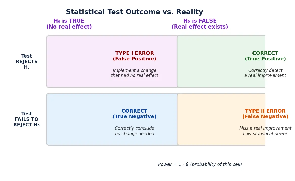
A test can therefore be statistically rigorous about false positives but still have low power. In that case, a non-significant result doesn’t necessarily mean the variation had no effect. It can mean the test didn’t have enough data to detect one.
💡Power isn’t a fixed property of your test
Power isn’t a single fixed property of an experiment; it is defined for a specific design and effect size. The power you set depends on your sample size, baseline conversion rate, significance threshold, outcome variability, traffic allocation, and the effect size the test is designed to detect. Smaller effects generally require larger samples to achieve the same power.
The four factors that determine whether your test has enough power
Statistical power comes down to four factors: sample size, MDE, significance level (alpha), and data variance. To see how these factors affect power, let’s use a scenario.
Imagine you run an online store. You want to test a new, bright green “Buy Now” button against your current gray button to see if it increases sales. By default, you set up a standard test: a 95% Confidence Level (Alpha = 5%), aiming for 80% power.
Here’s how each individual factor changes your test’s power:
1. Sample size (N)
Sample size is the total number of independent randomized units – usually unique visitors or users in an A/B test.
- A larger sample reduces the influence of random fluctuations and increases power.
- A smaller sample produces more uncertainty and makes false negatives more likely.
Say, you run the test on your online store. If only 100 people see the test over two days, a sudden burst of sales on the green button could easily be a fluke, like a single customer buying in bulk. Since the sample size is low, your test won’t have enough power to confidently tell a true lift from a coincidence.
However, if 50,000 visitors see the test in the span of a month, the random daily spikes will smooth out, and the test will have enough power to determine if the green button truly improved conversions or not.
2. Effect size (or minimum detectable effect (MDE))
The minimum detectable effect, or MDE, is the smallest improvement or decline that you want the test to reliably detect. It is the effect size at which the design reaches its target power. Smaller effects are not impossible to detect, but the test is less likely to detect them reliably at the planned sample. Larger effects are easier to distinguish from ordinary random variation, while smaller ones are harder to see.
- A larger MDE requires less data and gives the test more power at a given sample size.
- A smaller MDE requires more data because the test must separate a subtle signal from normal noise.
For example, if that green button boosts sales by 30%, the change is large enough that even a small amount of traffic gives your test enough power to detect it.
But if the green button only increases sales by 0.5%, that tiny change is easily hidden by normal daily variation in your traffic. To reliably detect a change that small, your test needs a lot more data (traffic).
If you set an MDE smaller than any change you could realistically produce, you either leave the test underpowered or require it to run for an impractically long time.
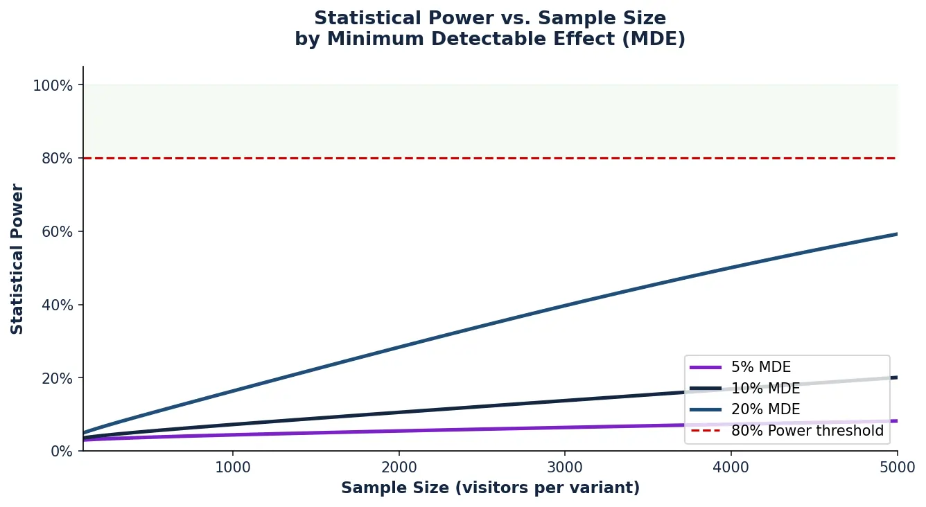
Here’s a diagram of how statistical power affects sample size for three relative MDE levels (5%, 10%, and 20%) at 5% baseline CVR and alpha = 0.05.
3. Significance level (α)
Your significance level, α, is the evidence you require before declaring a result statistically significant. A lower α (alpha) means you’re being more cautious about calling something a winner when there’s no real difference.
That caution comes with a tradeoff:
- A stricter, lower alpha makes false positives less likely, but also makes true effects harder to detect, which lowers power unless you collect more data.
- A more permissive, higher alpha makes effects easier to detect and raises power, but it increases the risk of false positives.
At the start of your test, you set the significance level to 5%. In this state, you require a reasonable amount of evidence to declare a winner, which leaves the test with enough power to flag the green button if it’s genuinely better.
But if you lower α from 5% to 1%, the test now strictly guards against false positives. It becomes overly cautious, so it will reject borderline results that might be true wins. That extra caution lowers your power to detect a real lift.
4. Data variability (variance)
Variance is the amount of natural fluctuation, or “noise,” in your data. In A/B testing, it’s closely tied to your baseline conversion rate and the standard deviation of metrics like revenue.
Here’s how variance affects power:
- Lower variance makes a true effect easier to detect and increases power.
- Higher variance makes the effect harder to separate from random noise and calls for a larger sample.
For example, say you test the green button on a subscription product priced at $10/month, then on a jewelry store where order values swing anywhere from $5 to $5,000.
With the subscription product, every buyer pays the same $10, which limits variation in order value. Revenue per visitor still varies between $0 for non-buyers and $10 for buyers, but it is less dispersed than in the jewelry example.
But with the jewelry store, order values vary widely. A visitor could buy $20 earrings and another could buy a $3,000 wristwatch. That variance reduces the power and makes it much harder for the test to detect the true effect of the button.
How to run a power analysis before your test launches
Running a power analysis before your test launches ensures you don’t waste time running a blind experiment. It tells you exactly how much traffic you need and how long the test must run to get a reliable result.
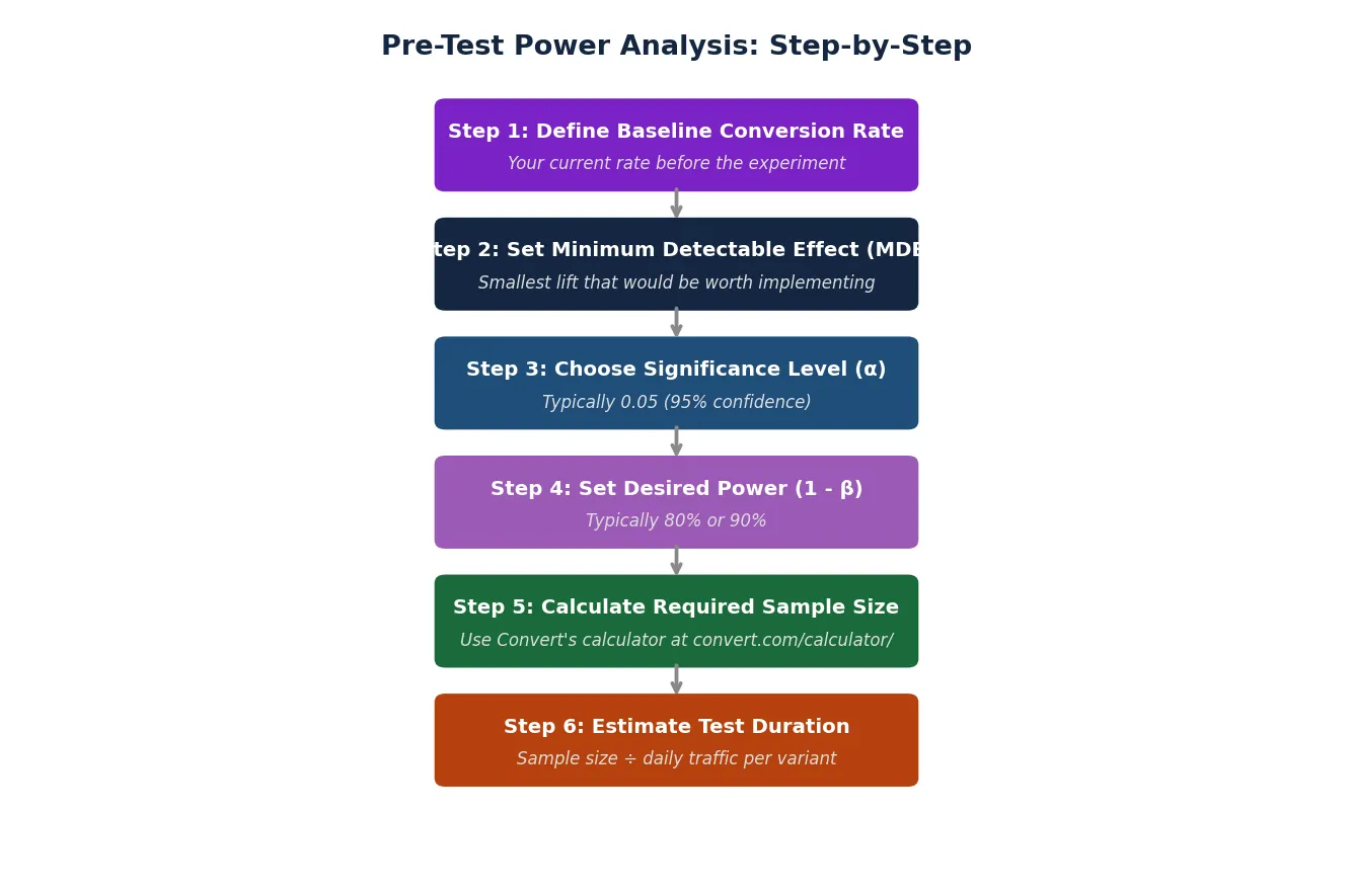
Here are the six steps to run a power analysis before conducting a test:
Step 1: Establish your baseline conversion rate
Your baseline conversion rate (CVR) is the current conversion rate of the control, before you change anything. This baseline is the foundation for all the calculations that follow, so use your own historical data rather than an industry benchmark.
Take the metric you plan to test (purchases, signups, add-to-carts) over a recent window, like the last 30 to 90 days. Divide the conversions by total visitors to get your rate. For example, if 5 out of every 100 visitors purchase, your baseline CVR is 5%.
A few things to keep in mind:
- Match the window to your cycle: If your traffic or sales swing by day of week or by season, pull enough historical data to cover a full cycle. A baseline taken from one unusually strong week will throw off everything downstream.
- Segment if your test targets a segment: If you’re only testing mobile checkout, use the mobile checkout conversion rate, not the site-wide average.
- Exclude anomalies: A flash sale, an outage, or a bot spike can distort the rate, so remove those first before you settle on the number.
Step 2: Set your minimum detectable effect (MDE)
Your MDE is the point at which a result becomes big enough to matter to you, so set it based on what would actually change your decision, rather than the lift you’re hoping for.
Keep in mind that a smaller MDE catches subtler wins but needs far more traffic, while a larger MDE needs less traffic, but it can miss smaller changes that would still have been worth shipping.
You can express your MDE in one of two ways:
- Relative MDE: A percentage of the baseline. A 10% relative lift on a 5% baseline means detecting a lift from 5% to 5.5%.
- Absolute MDE: A flat percentage-point change. A 10% absolute lift on a 5% baseline means detecting a lift from 5% to 15%.
Pro tip: Check which one your calculator or testing tool assumes. Setting a relative MDE in a tool that expects an absolute one (or the reverse) will give you a sample size estimate that’s off by a wide margin.
Step 3: Choose your target significance level (alpha)
Your significance level, α, is the risk of a false positive you’re willing to accept, or the odds of declaring a winner when nothing actually changed.
The standard is 5% (a 95% confidence level). Across repeated tests where the null is true, an α of 5% means about 1 in 20 will be significant by chance. Most tests use this, and it’s a reasonable default unless you have a reason to change it.
When you might adjust it:
- Lower α (1%): Choose this when a false positive would be costly, like when the winning change is expensive to roll out or hard to undo. You’ll need more data to keep the same power.
- Higher α (10%): Choose this when a wrong call costs little and speed matters more, like an early test you plan to confirm later. You get by with less data but accept more false positives.
Note: If you’re testing more than one variation, you also need to adjust α for the number of comparisons. Testing four variations against one control means four separate comparisons, and each one carries its own 5% chance of a false positive. Without a correction, the combined chance of a false positive across all four climbs well above 5%.
Step 4: Set your desired statistical power
Power is the probability that your test will successfully detect a true effect when one exists.
The standard default is 80%, which means that a variation that truly beats the control will be detected 80% of the time. The other 20% of the time, the test misses the win and comes back inconclusive.
Although most tests set power at 80%, you can aim higher when detecting an effect is critical:
- 90% power: Use this when the cost of missing a genuinely worthwhile effect is high. If the main concern is shipping an expensive or harmful false positive, use a stricter significance threshold or an explicit loss-based decision rule.
- 95% power: Reserve this for unusually high-stakes decisions where missing a true effect has severe consequences, alongside the domain-specific design and validation those decisions require.
💡 Pro tip: The higher your power, the larger the sample you need. So, set your target by weighing the cost of a missed winner against the traffic you have.
Step 5: Calculate the required sample size
With the first four numbers set, you can calculate the sample size needed to satisfy your parameters. But you won’t do this by hand.
Instead, input your baseline conversion rate, MDE, significance level (α), and power into a statistical power calculator, and the mathematical formula will output the number of visitors each variation requires.
Note that calculators usually report visitors per variation. For a test with one control and one variation, double that figure to get the total traffic you need across both.
💡 Pro tip: If the required sample is larger than your traffic can realistically supply, raise the MDE or lower your statistical power to bring the number down.
Step 6: Estimate your test duration
Duration tells you how long it takes to collect your required sample, based on the traffic you get.
To estimate test duration, divide your total required sample by the number of eligible visitors you get per day, and you’ll have the number of days the test needs to run. For example, if you need 40,000 visitors total and the tested page gets 2,000 visitors a day, the test runs for about 20 days.
Some things to note:
- Run for full weeks: Traffic and buying behavior shift across the week, so whole seven-day blocks improve representativeness and capture day-of-week differences in the treatment effect.
- Account for traffic split: If you send only half your visitors into the test, it takes twice as long to reach the required sample size.
- Watch the minimum runtime: Even with heavy traffic, run for at least 1–2 full weeks so the test captures a normal cycle rather than one unusually busy period.
Pro tip: Decide on the end date before you launch and stick to it. Ending a test early because the result looks significant is peeking, which raises your false positive rate above the α you set in Step 3.
💡 Try Convert’s A/B testing calculator
Instead of working the math by hand, plug your numbers into Convert’s calculator. Enter your baseline conversion rate, MDE, confidence level, desired power, traffic, allocation, and number of variations, and it estimates:
● The visitors required per variation
● How long the test is likely to run
● Which effect sizes are realistic for the traffic you have
● How the detectable effect shrinks as your sample grows
This gives you a realistic picture of what your traffic can and can’t detect before the test goes live.
The true cost of running underpowered tests
Underpowered tests do more damage than simply “missing a few winners.” Low power also costs you money and, worse, directly undermines the trustworthiness of the winners you actually find.
Here’s how:
The financial cost of an underpowered test
Suppose a SaaS business generates $1 million in monthly revenue at a 5% baseline conversion rate.
The product team designs a test for a new checkout flow. They want a fast answer, so they set a large relative MDE of 10% to keep the required sample size low. At that MDE, the test is well-powered to detect a lift from 5% to 5.5%.
The new checkout flow is a success, but it produces a modest 2% lift, which moves conversion from 5% to 5.1%. Since the test was only sized to catch a change as large as 10%, it lacks the power (sensitivity) to notice a 2% change. When the test finishes, the report reads “not statistically significant,” and the team interprets that as “the idea didn’t work” and discards it.
In monetary terms, a 2% lift on $1,000,000 is $20,000 in lost revenue every month. Over the course of a year, that single underpowered test costs the company $240,000 in unrealized growth.
Because SaaS businesses rely on recurring subscriptions, that $240,000 is also missing from the company’s baseline Annual Recurring Revenue (ARR) going into the next year.
The takeaway: An inconclusive result does not have zero economic value. It may represent a profitable effect that the experiment was incapable of seeing.
Low power makes your “wins” less trustworthy
The subtler cost is that underpowered testing can contaminate the pool of statistically significant results.
Say you run 100 experiments, and in reality 50 of the variations have a true effect while the other 50 do nothing. You set your significance threshold at α = 0.10 and your tests run at only 10% power.
Among the 50 experiments where nothing is happening, the α threshold means approximately 5 will come back significant anyway. These are false positives.
Among the 50 that have a real effect of the size used in the power calculation, 10% power means you expect to correctly detect about 5 of them (true positives), while about 45 real effects go undetected.
You end up with 10 statistically significant results:
In expectation, half of the apparent wins in this simplified example are false, which puts the false discovery rate at 50%.
Note: Setting the significance level (α) to 10% doesn’t automatically make 50% of your winners false. Alpha controls the false-positive rate among experiments where no effect exists. The reliability of your winner list also depends on how many variations truly work and how much power you have to find them.
At a fixed significance level, low power does not create more false positives among tests where no effect exists. It creates fewer true positives among tests where effects do exist, so false positives can make up a larger proportion of everything that appears significant.
Convert has a simulator that shows you how the share of statistically significant findings expected to be false increases as power falls, and how MDE and sample size correspond while power stays constant.
The data it costs
▲ Rises with power
To reliably catch a 5% lift on a 10% conversion rate, you’d need…
—
visitors per variant
Assumes a two-sided test at 5% significance. Double this for total A/B traffic.
The smallest effect you can see
▲ Rises with power
If your traffic is capped at 5,000 visitors per variant, the smallest lift you can trust this test to catch is…
—
relative lift
Assumes a 10% baseline conversion rate and 5% significance. More certainty from fixed traffic = only bigger effects qualify.
The wins you can trust
▼ Falls with power
If 1 in 4 of your test ideas truly works, this share of your “significant wins” are false alarms…
—
of wins are fake
Assumes 5% significance across many tests. Low power shrinks true wins until false alarms dominate.
What happens when you increase the power?
The same setup at 80% power tells a very different story. The 50 null experiments still produce about 5 false positives, but the 50 real-effect experiments now detect 40 true effects rather than 5.
You end up with 45 significant results: 40 true positives and 5 false positives, so your false discovery rate falls from 50% to 11%.
Nothing changed except the power of the tests. This shows that statistical power affects more than the interpretation of non-significant results. It also affects how much confidence you should place in the significant results produced by your experiment.
Why do experts call Twyman’s on low-powered tests?
Twyman’s Law is a fundamental principle in data analysis that states that any figure that looks interesting or unusual is probably wrong.
When experts see a large “winning” result come out of an underpowered experiment, they tend to “call Twyman’s” on it, meaning the result could reflect sampling noise, effect-size exaggeration, or a collection, measurement, or tracking problem, so it deserves additional checks before rollout.
There are two reasons they do this:
- A high false discovery rate
As the 100-experiment scenario showed, low power corrupts the pool of significant results. If you run a batch of tests at 10% power and a 10% significance level, about half of the winners are expected to be false positives in this simplified scenario.
Since a random false positive is as likely to appear as a muted true positive, the “win” can’t be trusted. If experts go ahead and roll out that variation, the effect likely won’t show up in the real world.
- The winner’s curse
In an underpowered test, a true effect usually reaches significance only when random noise pushes the observed result higher.
Suppose the true lift is 1%, which is too small for your test to detect reliably. When this test reaches significance, it is often because sampling noise pushed the observed lift above its true value. When this happens, the 1% lift can show up as something far larger, like 10%. That estimate is likely exaggerated, so experts call Twyman’s on it rather than celebrate.
Note: Calling Twyman’s law doesn’t mean declaring the result false. It means changing the burden of proof:
“This result is unusually large relative to the test’s sample size, historical results, and plausible mechanism. We should assume that it may be noise or an implementation problem until it survives additional checks.”
Power across statistical methods (Frequentist vs. Sequential vs. Bayesian)
How you handle power depends on which testing method you use. Here’s what it looks like in frequentist, sequential, and Bayesian testing.
Frequentist
In a standard fixed-sample Frequentist test, you plan power before launch. You choose an MDE, alpha, and desired power, calculate the required sample size, and wait until you hit it before looking at results.
Here, power keeps its classical meaning: the probability that the test produces a significant result when the specified effect is real. Checking repeatedly or stopping the test early can cause the false positive rate to be higher than the α you chose.
The six-step process earlier in this piece is a Frequentist power analysis.
Sequential
Sequential testing is designed for continuous monitoring, so you don’t have to commit to one exact stopping point. The statistical boundaries adjust as data accumulates, which lets the test stop early once the evidence is strong enough.
While power is less tied to a single fixed sample, it’s not irrelevant. You still need to consider the effect worth detecting, your false-positive tolerance, the stopping rule and planned horizon, and the probability that the procedure will detect that effect.
Sequential testing can reduce the average sample in some designs, but it can’t make a small effect detectable with almost no data.
Bayesian
Bayesian analysis does not usually report “powered” versus “underpowered” as a formal threshold. Instead, it reports probabilities such as chance to win, along with risk or expected loss.
However, the same planning question still applies. You can simulate how often a Bayesian decision rule would correctly recommend a winner when different true effects exist. So Bayesian methods don’t remove the question of sensitivity. They just express and evaluate it through decision probabilities rather than through significance and power thresholds.
How to calculate power for non-conversion metrics
Many test analyses focus on a binary conversion metric: a visitor either converts or doesn’t. However, many decisions ride on non-conversion metrics like revenue per visitor (RPV), and those behave differently. Because visitors are the randomization unit, RPV is usually the primary revenue decision metric:
RPV = conversion rate × AOV.
AOV helps explain why RPV moved, but it should not normally replace it as the primary test metric.
RPV often has higher variance than a conversion rate because most visitors spend nothing while a few spend a lot. That variance can mean an RPV test needs a larger sample to reach the same power as a conversion test.
This is easier to see with real numbers, so I ran both metrics through Convert’s calculator.
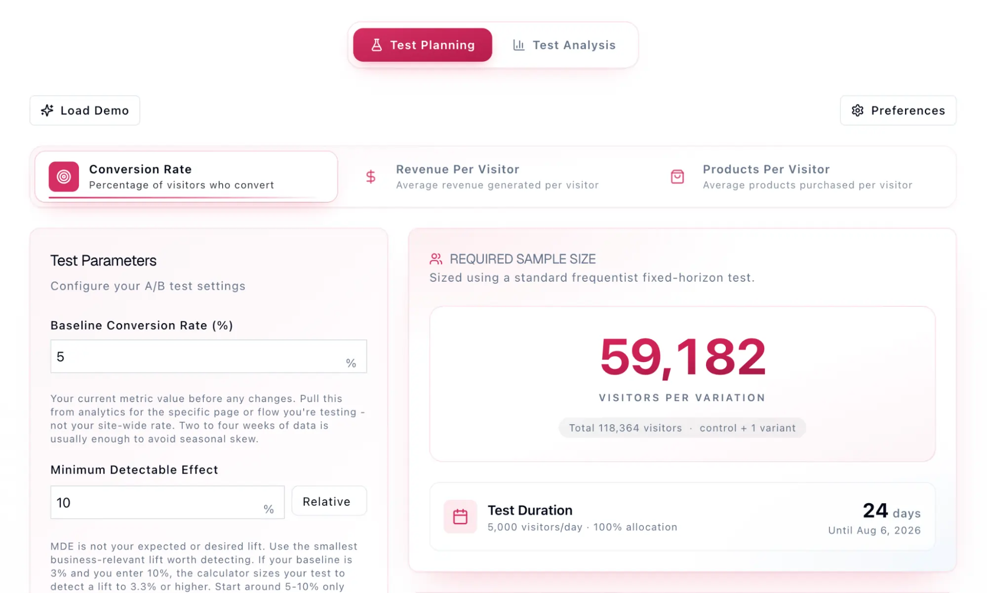
For the conversion rate test, I set up a two-sided frequentist analysis with one control and one variation, using 99% confidence and 90% power:
- 5% baseline conversion rate,
- 10% relative MDE
- 5,000 total daily visitors to the page
- 100% of traffic in the test
The calculator returned 59,182 visitors per variation, or 118,364 in total, with the test running for 24 days.
For revenue per visitor, I uploaded a CSV of all 5,000 visitors and their individual order values, with $0 for everyone who didn’t buy. The exact sample-size result depends on the spread of those visitor-level values, not just their average.
At the 5% conversion rate, revenue per visitor (RPV) came to $4.24.
Holding everything else the same – the same 10% relative MDE, 99% confidence, 90% power, two-sided test, 5,000 daily visitors, and 100% allocation, the calculator returned 105,323 visitors per variation, or 210,646 in total, and a runtime of 43 days.
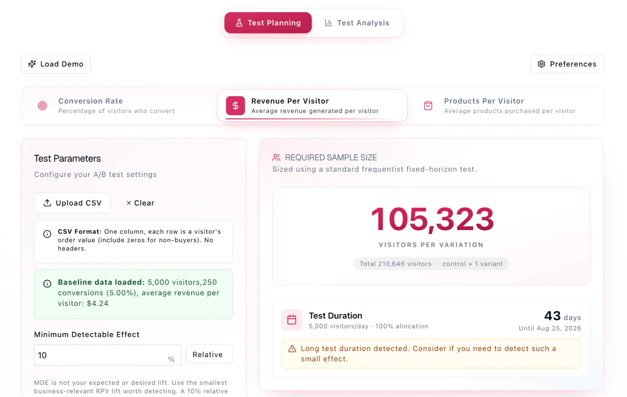
With the same MDE and the same traffic, the RPV test needed nearly double the sample and almost twice the runtime as the conversion rate test.
Why this happens, and how to size these tests
A conversion rate has a naturally bounded variance, since every outcome is a 0 or a 1. Revenue per visitor has no such limit.
A few large orders fall well above the $4.24 average, and the test has to see past that dispersion to detect a change. When a metric varies this much, you need more data to tell a true effect apart from the noise.
So sizing a test for a non-conversion metric like RPV depends on an input a conversion test doesn’t ask for: the standard deviation of the metric. Instead of a baseline rate, you supply the mean and standard deviation from your historical data, and the calculation uses that variability to work out the sample.
Metrics with a wider spread, like revenue or order value, may need more traffic than a bounded conversion rate at the same MDE.
What to do when you can’t achieve adequate power
The reality of experimentation is that many teams face traffic constraints that make running a test at 80% power to catch a 5% MDE a six-month commitment. For most businesses, keeping an experiment live for half a year is not feasible.
When your traffic can’t support a standard power analysis, you have to compromise. Here are four practical things you do instead (as well as their tradeoffs):
1. Increase your MDE
Instead of sizing your test to catch a small, subtle improvement, raise your MDE to detect larger improvements, like a 20% or 30% relative lift. When you increase your MDE, the required sample drops, which brings the runtime back in a reasonable range.
The simulator below shows how this plays out. As you change the MDE, the required sample changes while power remains constant.
The data it costs
▲ Rises with power
To reliably catch a 5% lift on a 10% conversion rate, you’d need…
—
visitors per variant
Assumes a two-sided test at 5% significance. Double this for total A/B traffic.
The smallest effect you can see
▲ Rises with power
If your traffic is capped at 5,000 visitors per variant, the smallest lift you can trust this test to catch is…
—
relative lift
Assumes a 10% baseline conversion rate and 5% significance. More certainty from fixed traffic = only bigger effects qualify.
The wins you can trust
▼ Falls with power
If 1 in 4 of your test ideas truly works, this share of your “significant wins” are false alarms…
—
of wins are fake
Assumes 5% significance across many tests. Low power shrinks true wins until false alarms dominate.
The tradeoff: When you increase the MDE, your test has less power to detect smaller but potentially business-relevant effects. So, if your variation creates a 5% lift, a test designed around a 20% or 30% MDE may not detect it reliably. Smaller effects remain unresolved rather than automatically disproved. Choose a large MDE only when effects below that threshold would not justify implementation, or when limited traffic means the experiment is explicitly a screen for very large effects.
2. Accept lower power
You can choose to leave your MDE at a realistic level (like 5%) but deliberately lower your target power from 80% down to 50% or 60%. Lowering the target power shrinks the amount of traffic you need, allowing you to conclude the test much sooner.
The trade-off: The lower your power, the higher your risk of false negatives. If you drop your power to 50%, you’re conceding that even if your new variation is a genuine winner, your test only has a coin-flip chance of successfully flagging it. In this case, record the power level next to the result, and treat any win as provisional until a stronger test confirms it.
3. Run the test in a high-traffic segment
Run the test on a higher-volume surface or broaden eligible traffic without changing the population the decision is meant to cover. If you deliberately restrict the audience to a segment, use that segment’s baseline and interpret the result only for that audience.
For instance, you might launch the test only for mobile users or on your highest-traffic landing page when that is the population you intend to serve. Restricting the audience does not create more traffic by itself; it changes who the result applies to.
The trade-off: You won’t be able to attribute results to the general website or traffic. A win among mobile users doesn’t mean the feature will work for desktop users. If you launch the winning variation site-wide later, it might underperform or even reduce performance on the un-tested segments.
4. Use sequential testing
With an unadjusted fixed-horizon frequentist test, you should not stop early just because a result becomes significant.
Sequential testing, however, uses an explicit monitoring rule that can allow valid early stopping when its boundary is crossed.
This framework sets stricter boundaries for significance early in the test. So, if your new variation delivers an absolute home run right out of the gate, the model allows you to stop the test early and claim a reliable win without invalidating the results.
The trade-off: Sequential testing does not guarantee a smaller sample. It may stop earlier when evidence crosses a valid boundary, but the sample-size benefit depends on the true effect and the stopping design. It does not make small effects detectable with little data.
Get statistical power right with Convert Experiences
Statistical power determines whether your test can detect an effect of the size it was designed for.
A well-powered non-significant result is more informative because it makes effects at or above your prespecified MDE less plausible, especially when the confidence interval excludes them. It does not prove that no effect exists; smaller effects may remain compatible with the data.
But if you get it wrong, that same result can’t be trusted, since the test was never sensitive enough to detect the effect in the first place.
That’s why it’s crucial to run a power analysis before every test. The goal isn’t only to produce a sample size, but to decide whether the test is worth running given your traffic, and what size of effect it can realistically detect in the time you have.
Convert’s sample size calculator does the math. Simply enter your baseline conversion rate (or upload a CSV file for non-conversion metrics), minimum detectable effect, confidence level, desired power, and traffic, and it returns the sample you need per variation and how long the test will run.
To get started, try out Convert’s calculator. And if you’re ready to run your test, start a free 15-day trial to see how Convert can help.


Mobile reading?
Althea Storm
Althea Storm is a B2B SaaS writer who’s worked with top companies like HubSpot, Thinkific, and Zapier to create content that informs and converts. She has a knack for making complex tech feel simple, useful, and genuinely engaging. When she’s not writing about software, she’s either reading fiction or working on some of her own.

How Was This Blog Written
This article was created by Althea Storm, Content Writer, with editorial review by Carmen Apostu,…
How Was This Blog Written
This article was created by Althea Storm, Content Writer, with editorial review by Carmen Apostu,…
This article was created by Althea Storm, Content Writer, with editorial review by Carmen Apostu, Head of Demand Generation.
To develop it, we used the following sources of input:
– Primary sources reviewed: Research papers, product documentation, discussions in forums and Slack channels.
– Internal expertise used: Data team
AI assistance was used for: Outline generation, image generation, and editing for clarity
AI was not used for: Final draft writing, product claims, source verification, final editorial approval
Every factual claim was reviewed by Althea Storm, Carmen Apostu, and Karim Naufal. Any claims involving statistical terminology were checked against Ron Kohavi’s papers on A/B testing and controlled experiments, and peeking and sequential testing.