Why 85% of Your Experiments Return Inconclusive (And the Fix)

Recently, a head of data analytics reached out after they saw one of my LinkedIn posts. He wrote, “We use home-grown A/B testing, but we always struggle with analyzing our tests. Most of them generate very low lifts. As a result, it’s always a very subjective decision what to do with the results.”

For most experimentation programs, this—low lifts, subjective decisions, mostly inconclusive results—is par for the course. And it’s not because the teams are bad at their jobs. It’s because the decision policy they inherited was never designed for their situation.

I wanted to see how bad the problem is, so I ran a simulation. In this simulation, the business was collecting 500 conversions over four weeks on the control version,  and there was a true underlying lift of +3.2% (that’s a real improvement, not a hypothetical one).

I ran that same experiment 100 times under identical conditions, and the only thing changing between runs was the random noise that characterizes the stochastic (random) nature of conversion rates.

The results: Under a standard two-sided 95% confidence interval (CI) policy evaluated at the four-week mark, 15 experiments reached a certification. The other 85 came back inconclusive.

An 85% inconclusive rate is a predictable consequence of applying a decision policy calibrated for a different problem.

So, the question to ask isn’t “How do we get to 95% confidence?”

It’s this: “Given the traffic we have, what policy actually produces decisions, and how do we increase our ability to ship winners without ignoring the risks of getting it wrong?”

When an experiment reports a lift of +8%, most practitioners read it as: “This variation is 8% better than the control.”

But that reading is almost certainly wrong.

Here’s what the experiment measured.

Over the specific days it ran, with the specific visitors it drew, the specific noise it encountered, and the exact sequence in which events occurred, the measured conversion difference came out to +8%.

If you run that same experiment again from the same underlying reality, you might see +2%. Or +14%. Or −3%.

The confidence interval already accounts for this mathematically. That’s why the result shows “95% CI: [+2%, +14%]” rather than just “+8%”.

The interval is there to describe exactly this uncertainty. But the number people remember, plan around, and forecast from is the +8%. The interval gets noted and forgotten, and the point estimate gets treated as the truth.

The stochastic path simulator I developed makes this impossible to ignore.

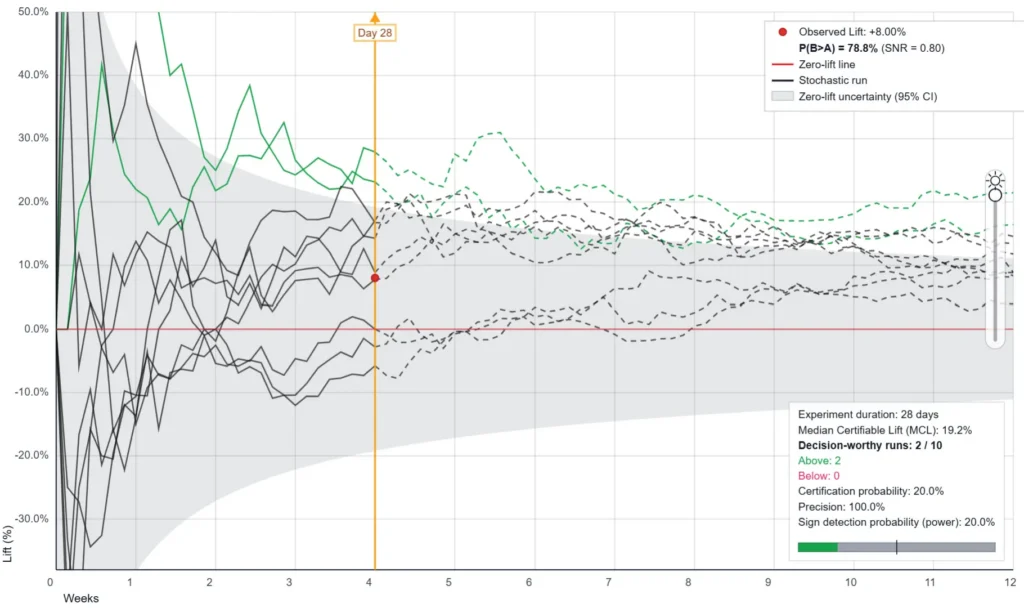
Each line on this chart is one possible path the experiment could have taken. They all share the same true underlying lift and start from the same reality, yet they still diverge wildly.

Some paths look strongly positive, some look very flat, some look negative, and while a few wander above the certification boundary, most don’t.

The line your experiment produced was one of these paths. You got a single draw from this distribution, and you never saw the rest.

This means two things:

1. The observed lift isn’t the true lift. The +8% you measured may be close to the true effect, or it may be a noise-amplified draw far above it. Or it could be a bad draw from a much higher lift. You simply don’t know, and you can’t tell with just one experiment.

   Strict thresholds only certify the paths that run extreme enough to cross a high boundary—which means they systematically select the hot paths.

   That’s why certified winners frequently underperform after launch. It’s easy to blame seasonality or implementation issues, but the likelier reason is that the policy certified an unusually high draw, and performance regressed toward the true effect once it was live.

2. You only get one shot. Frequentist statistics is built on the idea of infinite hypothetical repetitions, i.e., the p-value describes how a test behaves when it’s run infinitely many times under the null hypothesis.

   But in practice, you run the experiment once. You see one path and make your decision based on that path.

   What the simulation gives you is a map of the territory. It shows the realistic distribution of possible paths, so the decision policy you choose going in is designed for the entire distribution instead of the single path you happened to draw.

The double standard hiding inside your experimentation program

Here’s a question to ponder: A CMO approves a $100,000 campaign. The creative looks promising, the targeting feels right, and the timing lines up. What’s the probability that this decision is correct? 60%? 70%?

Nobody knows for sure, but the campaign launches anyway.

Another question: A product team ships a new onboarding flow. Customer interviews were positive, the mockups tested well, and the engineers are confident that the flow will improve activation. What’s the probability that they’re right?

Again, probably somewhere between 60% and 80%. No one knows for certain, but the feature ships.

We treat both of these as sound business decisions. Nobody demands certainty before launching a campaign or shipping a feature. Instead, the bar is: decent evidence, a manageable downside, and enough upside to make it worth a shot.

Then the same organization runs an A/B test, and suddenly 80% confidence isn’t enough. The team holds out for 95%.

But here’s what a lot of practitioners miss. A two-sided 95% CI (the standard threshold used by most testing platforms) works out to 97.5% one-sided confidence that B is truly better than A.

Before certifying B as the winner, it has to clear this very high bar. However, if you compare this experiment to other business decisions made at 60–70% confidence, then you’re holding your test to a bar almost 30 percentage points higher.

This is the double standard.

Everywhere else, the business adjusts how much confidence it needs based on what’s at stake. But experimentation doesn’t. It inherits one fixed number and applies it to every test, no matter the stakes.

That standard came from academic publishing, where a false claim can send other researchers down the wrong path for years. In that world, waiting for 95% confidence makes sense. But it wasn’t designed for things like a checkout page tweak or a headline test.

When you carry that same bar into business experimentation without asking whether it fits, you end up getting mostly inconclusive results.

Note: I’m not saying experimentation should be casual, or that you should drop your standards. My point is that the right standard depends on the decision — a change that affects every future visitor and is hard to walk back deserves more rigor than a one-off campaign bet, while a cheap, reversible test doesn’t need to clear the same bar. The goal isn’t less rigor. It’s matching the rigor to the stakes.

You already have a decision policy—whether you know it or not

Every test has a policy, whether the team chose it or not.

That policy includes:

• The threshold required to call a winner
• The minimum time the experiment has to run before any decision is allowed
• The maximum duration before the test expires, regardless of results
• How often the data is evaluated while the test is live
• What happens when the result comes back inconclusive

Each of these parameters shapes what your program produces.

For example, a strict threshold reduces your chance of a wrong call (a false positive), but it also misses more real winners, the ones that never cross that high bar. A lower threshold, on the other hand, catches more of those winners, but it’s more prone to wrong-direction calls (and calls winners with less magnitude bias).

Duration and monitoring work the same way. A test you run for four weeks will likely have different results than one you run for 12 weeks, and monitoring the test daily can yield different outcomes than a single end-of-test evaluation.

Most teams set these parameters once, from platform defaults to internal convention, and never revisit them. They simply run the test and wonder why they keep getting inconclusive results.

Before (re)running your test, ask: “What’s our decision policy? And given our traffic and baseline conversion rate, what’s it actually likely to produce?”

Remember the stochastic path simulator I built?

Rather than analyzing a single experiment, it replays the same experiment multiple times under identical conditions (same true effect, same traffic, same decision policy) and shows how the outcome distributes across all those possible paths.

I ran two scenarios through it, with identical inputs: 500 conversions on the control version over four weeks, a 3% baseline conversion rate, and a true underlying lift of +3.2%.

There were 100 simulated paths per scenario, and the only difference was the decision policy.

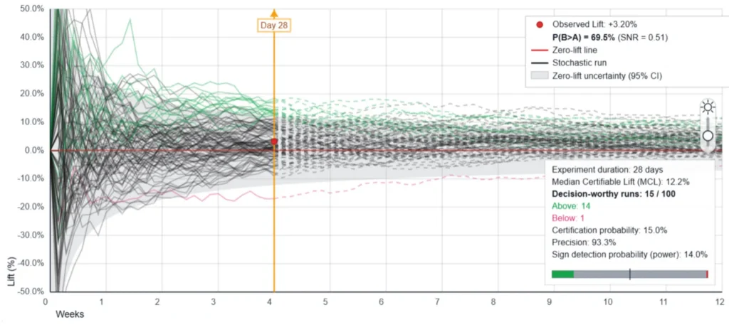
• 15 paths were certified—14 as winners and 1 as a loser. The other 85 remained inconclusive.
• The sign detection probability (i.e., the share of all 100 experiments that correctly identified the true positive effect) was 14%.
• Precision (i.e., the share of certifications pointing the right direction) was 93.3%.

This policy requires a true lift of at least 12.2% before it has even a 50% chance of certifying a winner. We call this the Median Certifiable Lift, or MCL, and I’ll come back to it below.

The true lift in the simulation, however, was 3.2%, well under that threshold, which means that the policy was not designed to see effects this small within a four-week window.

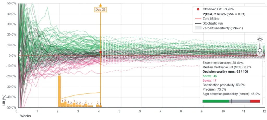
• 63 paths were certified—46 as winners and 17 as losers. 37 remained inconclusive.
• The sign detection probability climbed to 46%, up from 14%.
• Precision dropped to 73.0%, down from 93.3%.

The MCL here is 6.2%. That’s still above the 3.2% true lift, which is why sign detection is 46% rather than higher, but it’s close enough that the experiment identifies the real improvement in almost every other run.

What those numbers mean side by side

Under 95% CI, the program correctly identifies a real winner in about 1 out of every 7 experiments. But under SNR = 1 with daily monitoring, it correctly identifies a real winner in almost 1 out of 2.

An improvement from 1 in 7 to 1 in 2 shows that the program is gradually becoming a growth engine.

However, there is a precision cost. As we’ve seen, precision falls from 93.3% to 73.0%. So out of every 10 certifications under the lower threshold, roughly 3 point the wrong direction instead of 1. That’s the price of the lower threshold.

Now, the economics. Say you run 50 experiments a year:

• Under 95% CI, with 15% certification probability and 93.3% precision, the sign detection is 14%. That’s roughly 7 correctly certified improvements per year.
• Under SNR = 1, with 63% certification probability and 73% precision, the sign detection is 46%. That’s about 23 correctly certified improvements per year.

You can see the tradeoff in the three-segment bar at the bottom of each screenshot.

• Green = correct certifications
• Gray = inconclusive
• Red = wrong-direction calls

Under 95% CI, you get a sliver of green, a vast field of gray, and almost no red. It looks safe, but it’s mostly paralysis.

Under SNR = 1, there’s a substantial amount of green, a moderate band of gray, and some visible red. The risk is there, and you can see it clearly.

How to manage risk (realistically)

So how do you put this to work? Lowering the threshold blindly isn’t the move. What you want is to make the tradeoff visible and then choose it consciously.

Here are four ways to move from inherited defaults to deliberate policy design.

1. Know your sign detection before you launch

Before you ask “How many users do I need?”, ask a different question:

“Given my actual traffic, baseline conversion rate, and a realistic duration for this test, what sign detection probability does my current policy produce?”

Sign detection probability = Certification probability x Precision

At 14%, your program is set up to fail most of the time. But the culprit here is poor planning, not poor data. 

The Median Certifiable Lift, or MCL, is the most useful planning number. It’s the true lift at which your policy has a 50% chance of certifying a winner, and it’s determined by your traffic, baseline conversion rate, threshold, and monitoring cadence, so you don’t have to assume an expected lift up front.

For example, say your MCL is 12% and the effects your program typically generates are in the 3-5% range. Most of your experiments will come back inconclusive no matter how well you design them. Knowing that before you launch is more useful than discovering it four weeks later.

2. Run the negative scenarios before committing to a policy

The biggest risk of lowering your threshold is the possibility of certifying a small negative effect as a winner.

For most companies, tiny effects (smaller than 2% in absolute terms) are nearly impossible to detect in a typical 4- to 8-week test. Also, their impact is so small that chasing them is more of an academic debate than a practical business decision. 

Effects in the −3% to −5% relative lift range are close enough to zero that their paths wander above the certification boundary often enough to be called winners. But they’re big enough to hurt the business, so you should scrutinize them carefully.

Before committing to a lower threshold, simulate what happens when the true lift is −3%, −5%, and −8% relative, and ask: “What fraction of certifications point the wrong way in each scenario?”

 A −10% true lift generates strong negative evidence and rarely gets miscertified. But a −3% true lift is the danger zone because there’s a chance of it being called a winner.

If precision stays above 70-80% across all three negative scenarios, the policy is likely safe enough for most business contexts (but you have to do your own math here!).

3. Match the threshold to how reversible the decision is

Not every decision deserves the same threshold. The right bar depends on how easily you can walk the call back. Here are some examples:

• A headline test on a landing page: This is low stakes, reversible within days, and has limited structural fallout. Since the cost of making a wrong call is cheap and easy to undo, a lower threshold is appropriate.
• A significant pricing change: This affects every future customer and is difficult to reverse as it can confuse people and erode trust. Also, the cost of a wrong call is high and long-lasting. Since the expected effect is usually large enough to be certifiable at high confidence, a 95% CI is appropriate.
• A checkout redesign that reshapes infrastructure and creates technical debt: This is medium stakes and not easy to undo once it’s shipped. This one deserves deliberate policy design, probably something between 95% CI and SNR = 1, with a longer minimum runtime.

The threshold isn’t a fixed requirement, but a design choice that should follow the business risk of the specific decision being made.

4. Name and accept the precision tradeoff explicitly

If you lower the threshold, you and your team need to explicitly acknowledge that more certifications will point the wrong way.

That’s the agreed price of a higher-velocity program.

Document the policy before the experiment launches, in plain terms: “Under this policy, approximately 73% of our certifications will be correct. We accept the remaining 27% as the cost of a program that correctly identifies a winner almost every other experiment instead of every seventh experiment.”

Stating this clearly prevents:

• The team from panicking when a certified winner underperforms; and
• Stakeholders from citing a wrong-direction call as proof that experimentation “doesn’t work.”

What changes in practice

As I’ve mentioned earlier, the question that should kick off every experiment should be: “What’s our decision policy, and given our constraints, is it likely to produce the decisions this business actually needs?”

This question requires you to:

• Understand the policy before trusting the verdict;
• Simulate your expected outcomes before committing traffic; and
• Document what you’ve accepted before interpreting the results.

From there, here are some things to pay attention to:

1. Your inconclusive archive probably contains real winners

   If you’ve been running experiments for over a year under 95% CI, you’re likely sitting on a pile of inconclusive results. Under a lower threshold, a meaningful subset of those experiments contained a real signal that the policy was too strict to certify.

   Go back and re-evaluate those experiments under a lower threshold, and some of those winners will surface. The value has already been paid for in traffic and it can still be recovered.

2. The program compounds faster

   In keeping with our example from the simulations I ran, under 95% CI at typical business traffic levels, a program running 50 experiments per year ships roughly 7 correctly certified improvements.

   Under SNR = 1 with daily monitoring, roughly 23 improvements.

   That difference compounds over time, not because the lower threshold is more accurate per call, but because accuracy per call isn’t the only thing that matters.

   The number of correct improvements shipped per year matters, too, and a program shipping 23 winners per annum has a larger competitive advantage than a program shipping only 7.

Design the policy, then run the test

If your team can launch a $100,000 campaign at 60% confidence, ship a product at 70%, and redesign a pricing page at 65%, then you shouldn’t require 97.5% one-sided confidence before acting on an A/B test result.

If you do, this double standard will cause you to miss real winners, amass an archive of inconclusive tests, demoralize your team, and lose stakeholder trust because your experimentation programs appear to produce nothing.

To prevent (or fix) this, try to understand what your decision policy will produce under your constraints (traffic, baseline conversion rate, certification threshold, and monitoring cadence), explicitly state the tradeoffs, and pick the policy that serves the business best.

Ideally, your program should manage false positives, missed winners, and inconclusive results consciously, rather than optimizing for one at an unknown expense to the others.

That’s the standard experimentation should aspire to.

Clarifications for statistical purists

“But the example experiment was underpowered. A proper power analysis would have shown this.”

Correct, and that’s exactly the point.

The experiment is underpowered by classical standards. But if you run the power analysis for a 3.2% relative lift at a 3% baseline, it returns a required sample of approximately one million conversions.

At 500 conversions every four weeks per arm, that would take roughly 40 years. The objection is mathematically valid and practically useless.

The question is not whether the experiment satisfies a textbook ideal. It’s what policy gives you the best tradeoff under the constraints your business has.

“MCL is just MDE with a different name.”

Not quite. MCL is a specific, informative case of MDE: it’s the MDE at 50% power.

Conventional MDE is usually computed at 80% power (the effect size a test has an 80% chance of detecting). But MCL is computed at 50% power by definition, which is why “median” is the right word: half the stochastic paths certify, half don’t.

Both concepts share the same underlying structure but differ in what goes in and what comes out.

MDE requires specifying an expected lift before you know it (a number you have to guess and usually guess wrong). MCL asks only for your actual constraints, such as traffic, baseline conversion rate, certification threshold, and monitoring cadence.

In other words, MDE is a planning input derived from a hypothetical effect size, while MCL is a policy output derived from your real constraints.

MDE returns a required sample size; MCL returns a probability curve showing what your policy can see at any given duration. They answer different questions.

“Lowering the threshold inflates the false positive rate. That’s statistically indefensible.”

The false positive rate does increase, and this article names it explicitly.

Under SNR = 1, the theoretical false positive rate for the upper winner call at zero true lift is about 16%, compared to 2.5% for a two-sided 95% CI (one-sided). That cost is stated clearly.

The article also shows how to measure false positive risk across small negative true lifts (the practically dangerous scenarios) instead of only at zero.

A higher false positive rate isn’t indefensible when the full tradeoff, including missed winners and the organizational cost of inconclusive results, is made visible and accepted explicitly.

“Peeking at the data invalidates the statistical properties of the test.”

Under a 95% CI with fixed-horizon assumptions, repeated evaluation does inflate the false positive rate past the stated level. This critique of peeking is valid for that specific protocol.

However, the scenario in this article uses a pre-specified continuous monitoring protocol with a minimum observation period and a lower threshold—a completely different policy evaluated on its own terms through simulation.

The stopping rule is written into the policy from the start, not bolted on afterward. Simulation evaluates the full protocol and shows how it actually behaves, rather than assuming properties that hold only under fixed-horizon analysis.

“Sign detection probability isn’t the same as statistical power.”

Correct. Classical Neyman-Pearson power is defined for a specific protocol: fixed α, fixed sample size calculated in advance, and a single endpoint evaluation.

This article uses “sign detection probability” instead of “power” precisely for that reason. Sign detection probability is the generalization—the probability of certifying the correct direction of a true effect under any specified decision policy.

Classical power is the special case where the policy matches the textbook protocol. The two are compatible: sign detection probability subsumes classical power, but it doesn’t replace it.

“SNR = 1 has no established statistical justification.”

SNR = 1 is the natural boundary where the estimated signal equals the estimated noise. Under a normal approximation with a weakly informative prior, it corresponds to approximately 84% one-sided posterior probability that the true direction is positive.

It isn’t arbitrary; it’s the first point where the data gives you meaningful directional information. And the 95% CI has its own specific origin (Fisher’s conventions for scientific publishing), so it’s no more justified from first principles than SNR = 1 is.

Both are calibration choices.

The argument throughout is that teams should make those choices deliberately, based on business context, instead of inheriting them unexamined.

“You’re comparing a fixed-horizon test against a sequential testing protocol. That’s not a fair comparison.”

No. The comparison is between two complete decision policies applied to the same underlying experiment.

Policy 1 is a two-sided 95% CI with a single evaluation at day 28 and no peeking. Policy 2 is SNR = 1 with a 14-day minimum observation period, daily evaluation after that, and a four-week maximum.

Both are fully specified and are evaluated through simulation under identical true-effect and traffic conditions.

What’s being compared is their operating behavior (certification probability, precision, sign detection probability, and false positive profile), not their adherence to any statistical tradition.

A business choosing between decision policies should compare their operating behavior under realistic conditions.

“The 3.2% true lift example is cherry-picked.”

The example uses about  1000 total conversions at a 3% baseline over four weeks, which is a realistic window for a small-to-medium business.

The qualitative pattern (that 95% CI produces mostly inconclusive results for small-to-moderate effects at typical business traffic, and SNR = 1 with continuous monitoring improves sign detection substantially at a known precision cost) holds across the full grid of effect sizes and traffic levels in the simulator.

The specific numbers change, but the direction of the tradeoff doesn’t.