What Is the Bonferroni Correction in A/B Testing?


Let’s set the stage.
A CRO team runs an A/B/n test with one control and four variations, tracking three success metrics across each layout. One metric on Variant C clocks in with a p-value of 0.04. The team declares a winner, ships the change, and waits for the revenue to roll in.
But it never does. What went wrong?
The team fell victim to an invisible statistical trap: the multiple comparison problem.
By tracking three metrics across four variants, they were running 12 separate comparisons. If those 12 tests were independent and each used a 5% significance threshold, there would be about a 46% chance of at least one false positive—even if none of the changes had a real effect.
One way to reduce this risk is the Bonferroni correction, which sets a stricter significance bar across a planned family of comparisons. It limits the chance of at least one false positive, but it cannot guarantee that a result will replicate.
This article will break down how the Bonferroni correction works, when to use it in A/B testing, some Bonferroni alternatives, and which mistakes to avoid.
The multiple comparisons problem: Why more testing means more falsehoods
When you set up an A/B test, you choose a significance threshold, known as alpha (α). By convention, this is usually set at 5%, or 0.05.
That 5% threshold represents the false positive risk you’re willing to accept. It means: “If there is no real difference between the control and the variant, I accept a 5% chance that the variant will appear successful purely due to random coincidence.”
This mistake is called a Type I error, or a false positive.
If you only run one test, a 5% risk is easy to accept. The problem begins when you apply that same 5% threshold separately to several comparisons.
The explosion of risk: Family-Wise Error Rate (FWER)
Suppose you test one control against several variants. Or you compare one variant against a control but evaluate multiple metrics simultaneously.
The chance of getting a false positive doesn’t remain at 5% across the experiment. It rises as you add more tests. This is known as the multiple comparisons problem.
Statisticians measure this overall risk using the familywise error rate (FWER).
The FWER is the probability of getting at least one false positive across an entire “family” (or group) of tests you’re running.
When the tests are independent, you can estimate it using this formula:
FWER = 1 – (1 – α)m
Where:
- α is the significance threshold for each individual test.
- m is the number of comparisons being made.
The math in action
Here’s how quickly the FWER rises when multiple tests are run at the standard 5% significance level:
- 1 test: 1 – (1 – 0.05)1 = 5%
- 5 tests: 1 – (1 – 0.05)5 ≈ 22.6%
- 10 tests: 1 – (1 – 0.05)10 ≈ 40.1%
- 20 tests: 1 – (1 – 0.05)20 ≈ 64.2%
- 100 tests: 1 – (1 – 0.05)100 ≈ 99.4%
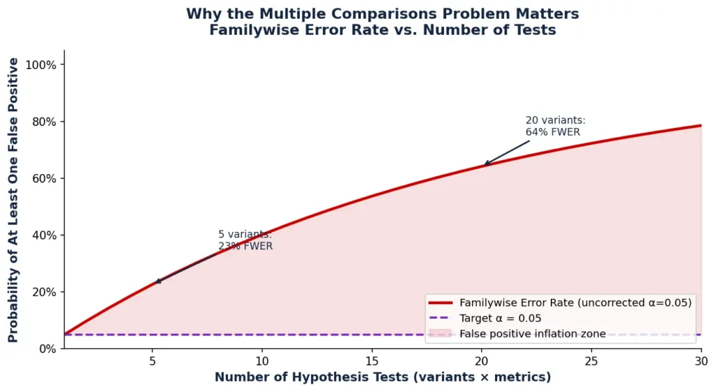
By 20 independent comparisons, there’s approximately a 64% chance that at least one will produce a false positive, even when none of the effects is real. At 100 comparisons, that becomes near certain (99.4%).
That doesn’t mean every statistically significant result is wrong. It just means that some of your apparent “wins” may simply be random fluctuations that happened to cross the significance threshold.
What the Bonferroni correction does (and the formula)
The Bonferroni correction gives you a simple way to account for the increased false-positive risk created by multiple comparisons.
Instead of testing every result against the usual 5% significance threshold, you divide that threshold by the total number of comparisons in the experiment. Each comparison then has a stricter bar to clear.
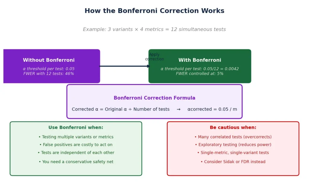
The formula is:
αnew (corrected alpha) = αoriginal ÷ m
Where:
- αoriginal is your baseline significance threshold (typically 0.05).
- m is the number of hypothesis tests in the family you want to protect.
- αnew (corrected alpha) is the strict new target value that an individual p-value must beat to count as statistically significant.
By making each test harder to pass, the Bonferroni correction keeps the FWER at or below your chosen level. If you want no more than a 5% chance of receiving at least one false positive across the whole experiment, Bonferroni divides that risk among the individual comparisons.
A worked A/B testing example
Suppose you’re running an experiment with one control, three variants, and two metrics. You compare each of the 3 variants against the control for both metrics.
That gives you:
3 variant comparisons × 2 metrics = 6 total comparisons
Without a correction, you would judge each comparison at an alpha of 0.05. But as we’ve seen, applying that threshold six separate times would increase your overall chance of finding at least one false positive.
Using the Bonferroni formula, you divide 0.05 by 6:
Corrected alpha = 0.05 ÷ 6 = 0.0083
Each result must now have a p-value below 0.0083 to be considered statistically significant.
For example:
- A p-value of 0.006 would be statistically significant.
- A p-value of 0.02 would not be, even though it would have passed the usual 0.05 threshold.
The second result may initially look like a winner, but it isn’t strong enough once you account for the six comparisons.
You can instead adjust each p-value by multiplying it by the number of comparisons (capped at 1.0), then compare it with the original alpha:
Adjusted p-value = original p-value × m
A p-value of 0.006 across 6 comparisons becomes:
0.006 × 6 = 0.036
Because the adjusted p-value is still below 0.05, the result remains statistically significant.
Note: Lowering alpha and adjusting p-values are equivalent when applied correctly. For transparency, report which correction was used and distinguish raw p-values from adjusted p-values.
When to use Bonferroni in A/B testing
Because the Bonferroni correction is highly conservative, applying it indiscriminately can starve your experiments of statistical power, causing you to miss out on winning product changes.
Here are the situations where it’s the right call:
1. You’re testing multiple variants against one control
Bonferroni is a great fit here because every additional variant creates another opportunity to declare a false winner.
The risk becomes more serious when a false positive would lead to an expensive rollout, such as:
- Rebuilding part of your product
- Changing your pricing or checkout flow
- Launching a new campaign across several markets
In these cases, applying a stricter significance threshold can help you avoid investing time and money in a result that may not be real.
2. You’re evaluating several primary metrics
The multiple comparisons problem doesn’t apply only to variants. It also appears when you test the same variant across several metrics. For example, you might measure whether a new product page affects conversion rate (CVR), revenue per visitor (RPV), and products per visitor (PPV).
Each metric represents a separate hypothesis test. If you’re willing to declare the experiment successful when any one of them reaches significance, you need to account for all three.
3. You have a confirmatory mindset
Bonferroni is appropriate when the experiment is designed to confirm a specific hypothesis rather than explore a large set of possible effects.
In a confirmatory test, you’ve usually decided in advance:
- Which variants you’re testing
- Which metrics matter
- What result would justify shipping the change
You’re not looking through the data to see what appears interesting. You intend to make an important decision based on the outcome, so a stricter correction helps ensure the evidence supports it.
4. Even one false positive would be a serious problem
Bonferroni controls the probability of making at least one false positive across the entire group of comparisons.
That makes it appropriate when even a single incorrect conclusion would be costly or difficult to reverse — experiments affecting:
- Customer payments
- Legal or compliance requirements
- User privacy
- A major product redesign
- A large advertising or implementation budget
5. You have enough traffic to support a stricter threshold
Bonferroni lowers the significance threshold for every comparison. As a result, you’ll usually need stronger evidence and a larger sample before a result is considered significant.
That may not be a major problem if you have:
- High experiment traffic
- Large expected effects
- A small number of planned comparisons
- Enough time to let the test reach the required sample size
How to calculate your total comparisons (m)
When every variant is compared with one control across the same set of primary metrics, you can use this rule:
m = number of variants × number of primary metrics
Here, “number of variants” means the treatment variants and excludes the control.
For example, if you run a test with a control and 4 new design variations, tracking 3 primary success metrics, your total number of comparisons is:
4 variants × 3 primary metrics = 12 comparisons
Your corrected significance threshold would be 0.05 ÷ 12 = 0.0041.
Each of the 12 comparisons would need a p-value below 0.0041 to be considered statistically significant.
💡 Clearing the confusion: Does Bonferroni apply per metric, per variant, or both?
The answer is both.
The Bonferroni correction cares about the total number of opportunities you have to make a mistake.
If you test 4 variants using one primary metric, Bonferroni applies across the 4 variant comparisons.
If you test one variant using 5 primary metrics and would call the experiment a success if any metric wins, it applies across the 5 metric comparisons.
If you test 4 variants across 5 primary metrics, and any combination could lead you to ship a change, the correction applies across all 20 comparisons:
4 variants × 5 metrics = 20 comparisons
The key question is whether the comparisons belong to the same group of hypotheses and can influence the same decision.
If several results can independently give you a reason to declare the experiment successful, they should be corrected together.
When Bonferroni hurts more than it helps
By making the significance threshold harder to reach, the Bonferroni correction also increases the chance that you’ll miss a real improvement.
That trade-off can be worthwhile when a false positive would lead to a costly or risky decision. But in other situations, Bonferroni can be so cautious that it makes the experiment counterproductive.
1. It can reduce statistical power (and increase false negatives)
Statistical power is the probability that your test will correctly detect a real effect when one exists. When Bonferroni lowers your significance threshold, your test needs stronger evidence to declare a result significant.
Say you run a test with 1 control and 5 variants, where each variant is compared with the control using one primary metric. The number of comparisons (m) is 5.
With an overall alpha of 0.05, the Bonferroni-corrected threshold becomes:
Corrected alpha = 0.05 ÷ 5 = 0.01
A result that would have passed at a p-value of 0.03 now fails because it doesn’t meet the stricter 0.01 threshold.
By prioritizing control of Type I errors (false positives), Bonferroni can increase Type II errors (false negatives). That means you may fail to detect genuine improvements, creating a different kind of decision risk.
2. It inflates the required sample size
To maintain adequate statistical power under a Bonferroni-corrected alpha, you need a larger sample size.
Take our five-variant test as an example. Instead of α = 0.05, Bonferroni lowers the per-comparison threshold to 0.01. The resulting sample-size increase depends on your baseline conversion rate, MDE, target power, test type, and traffic allocation.
- A universal estimate such as 100,000 users per variant can be misleading without those inputs.
- Use a calculator with your experiment’s actual assumptions instead of relying on a universal traffic figure.
In general, the stricter threshold increases the sample needed to preserve the same statistical power, which can lengthen the test.
3. It overcorrects on highly correlated metrics
Bonferroni treats every metric as another chance to find a false positive, which is useful when the metrics measure very different things, like site speed and user referral rate. But in most digital experiments, your metrics are connected.
Take a checkout test that tracks both conversion rate (CVR) and revenue per visitor (RPV). When a user buys something, their purchase both counts as a conversion and adds revenue. So while CVR and RPV tell you different things, they’re driven by the same user behavior.
However, Bonferroni doesn’t account for this connection, so it overcorrects, tightening the significance threshold for both metrics as though they were completely separate, and reducing your chances of detecting a true improvement.
4. It can hide useful signals during exploratory testing
In early research or feature development, missing a real signal (a false negative) is often far more risky than chasing a false lead (a false positive).
Imagine testing 20 wild, innovative design ideas at a 0.05 significance level to see if any sparks user interest. If you apply Bonferroni, your significance threshold drops to a brutal 0.0025.
A result with a p-value of 0.03 would no longer count as confirmatory under that 0.0025 threshold—even if its estimated lift looked promising.
💡 Pro tip: Bonferroni is better suited to confirmatory tests, where the results will directly influence what you ship.
Exploratory tests can be run without a correction, but their results shouldn’t be treated as confirmed wins. Instead, use them to identify promising hypotheses, then validate those findings in a separate, properly powered experiment.
5. It can make the sample requirement and test duration unrealistic
The Bonferroni threshold becomes smaller with every comparison:
- 5 comparisons: 0.05 ÷ 5 = 0.01
- 10 comparisons: 0.05 ÷ 10 = 0.005
- 20 comparisons: 0.05 ÷ 20 = 0.0025
As the threshold drops, the test needs more data to detect the same effect.
Apply Bonferroni to a multi-variant test in a low-traffic environment, and the sample inflation can push the test past what the traffic will support. A test that would normally take two weeks at α = 0.05 can stretch to much longer at α = 0.01.
In fast-moving industries, waiting that long creates massive opportunity costs and leaves your team paralyzed.
You may be tempted to stop the experiment before it reaches the corrected sample size, but that will leave you with an underpowered test that’s unlikely to detect anything except a very large effect.
💡 Plan your Bonferroni-corrected test with Convert
When you run a multi-variant test, Convert’s A/B Testing Calculator can account for multiple comparisons. Choose Bonferroni, enter your test details, and the calculator will estimate the sample size and test duration you need.
This lets you see the practical cost of the correction upfront and decide whether your experiment has enough traffic to support the stricter threshold.
Bonferroni vs. Holm-Bonferroni vs. Šidák vs. Benjamini-Hochberg vs. Dunnett’s correction methods
When the strictness of the standard Bonferroni correction threatens to paralyze your research, you don’t have to abandon statistical control altogether. Statisticians have developed a spectrum of alternative correction methods that shield your data from errors in different ways.
The heavy hitters: Holm-Bonferroni vs. Benjamini-Hochberg
The two most common multiple comparison corrections are Holm-Bonferroni (also known as the Holm method or the Bonferroni-Holm method) and Benjamini-Hochberg (BH).
Both correct for multiple comparisons, but they operate under fundamentally different philosophies and protect against different mistakes. Both start by ranking all p-values from smallest (most significant) to largest (least significant). But from there, they diverge.
How Holm-Bonferroni works
Plain Bonferroni applies the same corrected threshold, α ÷ m, to every comparison.
Holm-Bonferroni is more flexible. It checks your smallest p-value against the strictest threshold, then gradually relaxes the requirement as it moves through the remaining results:
- The smallest p-value is compared with α ÷ m.
- The second-smallest is compared with α ÷ (m − 1).
- The third-smallest is compared with α ÷ (m − 2).
This continues until one result fails. Once a p-value fails, that result and every result after it are declared non-significant, regardless of how close they were to passing.
Suppose you run 4 comparisons and receive these ranked p-values:
0.004, 0.012, 0.030, and 0.200
At α = 0.05, the Holm thresholds are:
- 0.004 compared with 0.05 ÷ 4 = 0.0125: Passes
- 0.012 compared with 0.05 ÷ 3 = 0.0167: Passes
- 0.030 compared with 0.05 ÷ 2 = 0.025: Fails
The process stops there. The p-values of 0.030 and 0.200 are both treated as non-significant.
Holm still controls the probability of making even one false positive across the family, but it’s less punishing than plain Bonferroni because not every result has to clear the same ultra-strict threshold.
How Benjamini-Hochberg works
Instead of preventing any false positives, the Benjamini-Hochberg method controls the expected proportion of false positives among the results you declare significant – the false discovery rate (FDR).
After ranking the p-values, each receives this threshold:
BH threshold = (rank ÷ number of comparisons) × FDR level
Using the same 4 p-values from earlier (0.004, 0.012, 0.030, and 0.200) and an FDR level of 0.05, the thresholds are:
- Rank 1: (1 ÷ 4) × 0.05 = 0.0125
- Rank 2: (2 ÷ 4) × 0.05 = 0.025
- Rank 3: (3 ÷ 4) × 0.05 = 0.0375
- Rank 4: (4 ÷ 4) × 0.05 = 0.05
Benjamini-Hochberg then works from the bottom up, comparing your largest p-value directly against its threshold. If it fails, BH moves up to the next largest p-value, tightening the threshold slightly based on its rank position.
The moment the first p-value passes its designated threshold, the search is over. That metric is declared significant, and every single p-value above it (the stronger results) is automatically put in the “significant” bucket as well.
In this example, 0.200 is larger than 0.05, so it fails. But 0.030 is smaller than 0.0375, so it passes. That result and every smaller p-value are declared significant.
💡 What’s the difference between the Holm-Bonferroni and Benjamini-Hochberg methods?
The difference between these two methods comes down to the specific type of error they prevent.
● Holm-Bonferroni controls the Family-Wise Error Rate (FWER): This is the probability of making even one false positive across your entire family of tests. Because it limits the probability of one or more false positives across the family, it can suppress borderline results.
● Benjamini-Hochberg controls the False Discovery Rate (FDR): This controls the expected proportion of false positives among the results you declare significant. At a BH target of 0.05, the procedure controls the expected false-discovery proportion at 5% under its assumptions; it does not guarantee exactly five false positives in every set of 100 discoveries.
Neither method is universally superior. The choice depends entirely on your operational goals.
● For exploratory work where missing true effects is costly, Benjamini-Hochberg can preserve more power by controlling the expected false-discovery proportion rather than the chance of any false positive.
● For confirmatory decisions where even one false positive would be costly (like validating a medical drug), a familywise-error procedure such as Bonferroni-Holm may be more appropriate.
The specialized alternatives: Šidák and Dunnett’s
When your experiment features specific, structured relationships between variables, you can use specialized corrections like Šidák or Dunnett’s rather than relying on general sequential methods.
How the Šidák correction works
Šidák solves the same basic problem as Bonferroni: controlling the FWER across several comparisons. The difference is in how it calculates the corrected threshold.
Bonferroni uses:
αnew (corrected alpha) = αoriginal ÷ m
Šidák uses:
αnew (corrected alpha) = 1 − (1 − αoriginal)(1 ÷ m)
For 5 comparisons at an overall alpha of 0.05:
- Bonferroni alpha: 0.05 ÷ 5 = 0.0100
- Sidak alpha: 1 − (1 − 0.05)(1 ÷ 5) = 0.0102
Šidák gives you a slightly higher threshold, which makes it marginally easier for a result to reach significance. But as the example shows, the difference is usually small.
🚨 Note: Šidák works best when your comparisons are independent. In A/B testing, however, it’s common for several variants to share the same control and multiple metrics to be influenced by the same users.
So while Šidák gives you slightly more power than Bonferroni, it isn’t automatically the better option. Use it only when your comparisons are reasonably independent and you want strict FWER control without using Bonferroni’s slightly harsher threshold.
How Dunnett’s test works
In digital A/B/n testing, it’s common to be faced with a scenario where you’re testing multiple treatment groups (Variant A, Variant B, Variant C, and Variant D) against a single baseline Control.
You don’t care about comparing Variant A with Variant B or Variant C with Variant D; you only care about how each variant performs against the control.
Bonferroni applies a general penalty to the comparisons you include without modeling their shared-control correlation. Dunnett’s test instead uses that experimental structure and accounts for the fact that every comparison shares the same control-group data.
Because it factors in this shared correlation, Dunnett’s applies a less restrictive penalty than Bonferroni or Šidák, preserving your statistical power while safely keeping your FWER under control.
Here’s a comparison table showing how these correction methods stack up against one another:
| Name | What it is |
How it’s applied |
When it should be used |
||||||||||||||||||||
|---|---|---|---|---|---|---|---|---|---|---|---|---|---|---|---|---|---|---|---|---|---|---|---|
| Bonferroni | A simple, conservative FWER correction. | Divide the significance level (α) by the total number of comparisons (m) and apply the same threshold to every test. | Use it for a small, predefined family of tests where even one false positive would be costly. | ||||||||||||||||||||
| Holm-Bonferroni | A sequential, step-down procedure that controls FWER. | Rank p-values from smallest to largest, then test them from the top down against gradually relaxed thresholds, and stop at the first failure. | Use it for confirmatory tests where strong control of the chance of any false positive is required. | ||||||||||||||||||||
| Benjamini-Hochberg | A sequential, step-up procedure that controls FDR. | Rank p-values from smallest to largest, assign each a rank-based BH threshold, then test them from the bottom up until the first success occurs. | Use it for exploratory research or large hypothesis families where the main priority is maximizing discovery rather than preventing false positives. | ||||||||||||||||||||
| Šidák | A slightly less conservative FWER correction than Bonferroni. | Applies a single, fixed threshold (calculated with 1 − (1 − αoriginal)(1 ÷ m)) based on the exact probability of independent events. | Use it when comparisons are reasonably independent and you want slightly more power than Bonferroni while retaining FWER control. | ||||||||||||||||||||
| Dunnett’s | A specialized FWER procedure for comparing several treatments with one shared control. | Evaluate all treatment-versus-control comparisons together while accounting for the shared control. | Use it for multi-variant testing (A/B/n tests) where multiple treatments are compared exclusively against a single control. |
How Convert handles multiple comparison correction
Convert gives you three multiple-comparison options in the Frequentist settings panel: Bonferroni, Šidák, or None.
In Convert, go to your experiment’s Report, then open Actions → Stats and Settings → Frequentist. You’ll find the Multiple Comparison Correction setting there.
- Bonferroni is the strictest option. It lowers the chance of a false positive, but it can make real winners harder to detect. Use it when being wrong would be especially costly.
- Šidák also controls familywise error and is slightly less conservative than Bonferroni. It can provide a little more power, although its exact calculation assumes independent comparisons.
- None applies no correction. Use it when you’re making only one comparison, or when the test is exploratory and you’re comfortable with a higher false-positive risk.
Once selected, Convert applies the chosen correction automatically to the relevant Frequentist comparisons in the report. You don’t need to calculate it manually.
Mistakes even seasoned testers make with the Bonferroni correction
Under pressure to ship features or publish findings, it’s easy to misapply statistical adjustments.
Here are the most common mistakes seasoned testers make when using the Bonferroni correction and how to avoid them.
1. Conflating global metrics with independent test families
Testers may bundle every single metric tracked across a company into one massive Bonferroni correction. But this penalizes tests unnecessarily.
Corrections should cover the predeclared hypotheses that can support the same decision. Unrelated descriptive metrics can be reported separately, as long as they are not used as extra chances to declare a win.
2. Mixing raw and adjusted p-values
You can correct either the significance threshold or the p-values; both approaches lead to the same decision when applied consistently.
The mistake is presenting an adjusted p-value as though it were raw, or comparing an adjusted p-value with a corrected alpha. Label adjusted values clearly, keep raw values available for context, and compare like with like.
Here’s why adjusting α is the better move:
- Preserve individual context. Keep the raw p-value available alongside any adjusted value.
- Improve transparency. Label the correction and adjusted value so stakeholders can see how the decision rule changed.
- Communicate one rule consistently. For non-technical stakeholders, explain that multiple comparisons require a stricter standard, whether the report shows a corrected threshold or an adjusted p-value.
3. Correcting every tracked metric when only one primary KPI drives the decision
If you choose one overarching primary metric in advance (for example, revenue per visitor), the extra secondary metrics do not automatically expand that metric family—as long as they cannot make the experiment a win. You may still need a correction for multiple variation comparisons on the primary metric.
Secondary metrics act as guardrails, helping you catch negative side effects rather than decide whether to ship the variant. Including them in a Bonferroni correction would make the significance threshold unnecessarily strict, reduce statistical power, and increase the risk of rejecting a genuinely successful change.
4. Using Bonferroni as an excuse to skip proper sample size planning
Some teams may bypass upfront power calculations by assuming they can just run the test and use a Bonferroni correction at the end to stay safe.
As shown earlier, Bonferroni can inflate the required sample size. If you don’t plan for this traffic surge before launching the test, you’ll end up underpowered and may have to either run the experiment for months or abandon it altogether.
5. Applying the correction to post-hoc segmentation searches
Applying Bonferroni to a standard multi-variant test won’t protect you if you slice your data by dozens of different user segments (like geography, device, or browser) after the test concludes.
Post-hoc data dredging introduces massive false-positive risks that require specialized segmentation corrections or entirely new replication tests. Relying on initial variant correction creates a false sense of security while hidden false positives leak into your segmented data.
Keep false positives in check with Convert
Bonferroni helps protect your experiment from false wins by lowering the significance threshold as the number of comparisons increases. Other methods, including Holm-Bonferroni, Benjamini-Hochberg, Šidák, and Dunnett’s, make different trade-offs between error control and statistical power.
Convert natively supports both Bonferroni and Šidák corrections. Simply choose the method you want in your test’s Frequentist settings, and Convert handles the calculations automatically.
Want to see what that correction means for your experiment? Use Convert’s calculator to estimate the sample size required for your corrected multi-variant test. Then, when you’re ready to put it into practice, try Convert free for 15 days.


Mobile reading?
Althea Storm
Althea Storm is a B2B SaaS writer who’s worked with top companies like HubSpot, Thinkific, and Zapier to create content that informs and converts. She has a knack for making complex tech feel simple, useful, and genuinely engaging. When she’s not writing about software, she’s either reading fiction or working on some of her own.

Carmen Apostu
Content strategist and growth lead. 1M+ words edited and counting.
How Was This Blog Written
This article was created by Althea Storm, Content Writer, with editorial review by Carmen Apostu….
How Was This Blog Written
This article was created by Althea Storm, Content Writer, with editorial review by Carmen Apostu….
This article was created by Althea Storm, Content Writer, with editorial review by Carmen Apostu.
To develop it, we used the following sources of input:
– Primary sources reviewed: Research papers, product documentation, discussions in forums and Slack channels.
– Internal expertise used: Data team
AI assistance was used for: Outline generation, image generation, and editing for clarity
AI was not used for: Final draft writing, product claims, source verification, final editorial approval
Every factual claim was reviewed by Althea Storm, Carmen Apostu, and Karim Naufal. Any claims involving statistical terminology and correction methods were checked against Ron Berman’s paper on false discovery in A/B testing.